The ever-present ghost of data quality in SDMs

Those who know me are likely well aware of my interest in species distribution models (SDMs). In particular, I’ve been focused for years on how we can enhance these models using higher-resolution data, such as microclimate information or anthropogenic disturbance.

This queeste for increasing SDM-resolution, however, has to overcome a few highly important data-related issues that can’t be fixed by simply increasing the resolution of the maps used as explanatory variables. In a review published just now in Ecography, we discuss these and related issue: sample size, positional uncertainty and sampling bias. Indeed, one can have microclimate data with as high of a resolution as possible, if your species data is suffering from one of these three issues, you can’t get the performance of your model anywhere close to what you might have been hoping for.

Sampling bias, sample size and positional uncertainty – the three characteristics of the looming ghost of data quality that might affect the performance of your SDMs. All three of them are affected by species ecology and the environment.

Positional uncertainty

Case in point: positional uncertainty. When building SDMs, we often think about our species observations as points on the map. Often they are not, however; they are more like smudges. Depending on the data, the observational errors can range from just a few meters (e.g., GPS inaccuracies) up to a kilometer (e.g., aggregated data from global databases) or even more (e.g., historical data with poor location information such as some herbaria). Failing to take into account that uncertainty (i.e., working with the falsely comforting points rather than the smears on your map) could affect the apparent correlations between species observation and environmental data. The size and importance of this error also varies between species. For example, for mobile species it is often much harder to pinpoint an exact location, while deep-sea organisms are often located using less-accurate acoustic positioning.

Three categories of factors driving positional uncertainty: the resolution and configuration of the spatial predictors (e.g., micro- versus macroclimate data – see the paper for more details), recording techniques and data processing (e.g., GPS accuracy) and species ecology and site characteristics (e.g., a lower accuracy for big animals, limited GPS accuracy under forest canopies or in cities)

Sampling bias

A similar issue exists with sampling bias. Often enough, we feel reassured by big numbers, with models built using thousands of points looking soothingly trustworthy. Here again, however, these numbers could create false confidence.

Species observations often have strong spatial bias, with many points located close to each other, and big gaps in between. Typically, positive sampling biases have been reported towards easily accessible areas (e.g. proximity to roads, rivers, and urban settlements), protected areas, more populated areas, and charismatic species, leading to spatial and taxonomic biases. Uneven data-sharing practices make this issue even worse. These issues are not only present when using citizen science data, but at a larger scale also when using data collected by researchers, who are similarly biased towards certain locations that are more reachable, more interesting, or more likely to attract funding.

Clear recommendations

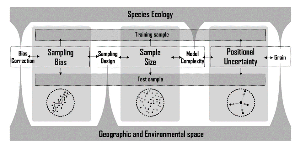
Importantly, our review goes beyond a simple discussion of these problems with our SDM-data. We made a point of creating clear, hands-on suggestions on how to deal with these issues, every step along the way. These suggestions are summarized in the figure below.

With that, we hope this review can become a helpful guide for anyone working in the amazing but treacherous world of species distribution modelling. With our review in hand, the data should not play further unexpected tricks on you!

Read the whole review and its recommendations here in Ecography.

Posted in Science | Tagged , , , , , | Leave a comment

Veronica

The series of papers known as ‘Geron et al.’ has a new addition, marking the final piece of Charly Geron’s PhD trajectory studying the link between urban plant invaders and urban microclimates.

In his earlier chapters, we already demonstrated that urban invaders often originate from warmer and drier native regions, probably benefiting from the warmer urban temperatures due to the urban heat island effects. We found that these species nevertheless prefer shaded environments, which protect them during urban heatwaves. We also explored the traits, phenology and genetics that contribute to these behaviors.

In the latest article by Geron et al. published in Oecologia, we delve deeper into the latter pressing question: do non-native plant species adapt to urban environments? We focused on the delicate little (but make no mistake, this species native to the north Caucasus and Iran can be a real crop pest) flower Veronica persica (bird’s-eye speedwell) as our model species, conducting a combination of field (or better – urban road verges and wastelands) surveys and a ‘common garden’ experiment.

What we were after was straightforward to articulate, but – sorry – bloody difficult to test: was there a difference in the development and performance of Veronica persica between urban and rural settings, and, if differences exist, could they be attributed to either adaptation, mother plant influence or simple plasticity? if plants from urban origin showed a higher reproduction in urban microclimate, it might be the sign of adaptation to urban environments. If not, it could suggest that Veronica persica is highly plastic, resulting in variations in its development following local conditions but not due to genetic changes.

Our findings highlighted the latter scenario. Veronica persica exhibited significant phenotypic plasticity across all measured traits, with reduced germination, growth, and flowering under urban conditions. This suggests significant setbacks to plant success in the more stressful growing conditions of a warmer urban microclimate.

Interestingly, we found no significant differences in how well urban versus rural plants coped with these conditions, indicating a lack of local adaptation. However, we observed notable genetic differences at the population level, influenced by the identity of the mother plant, suggesting genetic diversity among populations.

Strong phenotypic plasticity between rural and urban microclimates, with lower germination, longer germination delay, (substantially!) fewer flowers and longer flower delay in urban microclimates. No sign, however of local adaptation (red lines = urban origin, blue lines = rural origin, yet both colors are simply scattered randomly).

Does this mean that non-native plant species cannot adapt to urban environments? Certainly not. It’s important not to generalize based on a single species. Our findings did align surprisingly well with previous research on Matricaria discoidea (pineapple weed), however, which also demonstrated strong phenotypic plasticity and maternal effects, but no clear local adaptation.

Two is not yet a crowd, yet they do show clearly that detecting subtle local adaptation amidst the variability introduced by phenotypic plasticity is challenging, especially in highly adaptable ruderal non-native species.

We can only end – as so often necessary – with a call for further research. Urban environments are warming rapidly, and the urban environment creates unique ecosystems. Understanding how both non-native and native species may or may not adapt to these conditions is crucial for protecting future biodiversity.

Read the full story in Oecologia or here on ResearchGate to find out more!

Posted in Belgium | Tagged , , , , | Leave a comment

Tarfala

The Tarfala research station, with some of its beloved glaciers in the background

While a lot is going on in and around Abisko, as can be seen in yesterday’s story, part of the team has ventured further south, to the perhaps even more beautiful moonscape of Tarfala.

Here, a rugged mountain cabin hosts the research team studying some of Sweden’s tallest mountains and biggest glaciers.

For us, it is the vegetation in the glacier forefield that we care about: can we reconstruct the monitoring transect from a set of historical surveys and reconstruct how the vegetation has changed following the inevitable glacial retreat?

A helicopterflight or 24 km long hike away from the nearest road, Tarfala is clearly a notch more adventurous than the Abisko area!

Pictures by Jeanne Terragno

Posted in Sweden | Tagged , , , , , , , | Leave a comment

The summer is for Sweden

The group has a whole team up north again, monitoring vegetation and bumblebees, gathering microclimate data and so much more.

I was lucky enough to spend a few days up there as well, checking up on the long-term monitoring sites on mount Nuolja, hiking to the top of our gradient in the beautiful valley of Laktatjakka, and checking out the extremely poor and acidic heathlands of the steep slopes of the Norwegian fjord of Rombak.

Next week, a final two days of fieldwork for me in a beautiful Norwegian valley, then it’ll be the awesome, interested and enthusiastic students and fieldwork crew holding the fortress till early September and autumn setting in again. Jealous, but happy it’ll be a great time with great science for them!

Microclimate and vegetation monitoring with a view of Abisko village
A yellow field of buttercups
Absolute cutie: Linnaea borealis
The beautiful wooden poles marking our long-term vegetation monitoring plots on mount Nuolja, with the famous Lapporten mountain gap in the background
Evening sun on Trollius europaeus and Geranium sylvaticum
Microclimate monitoring with a view of a Norwegian fjord
This majestic rock has tempted to roll down into the fjord for at least twelve years
‘Vegetation’ monitoring in the high-alpine zone of the Laktatjakka trail
Ranunculus glacialis
Part of the team in action on a beautiful day in the Laktatjakka valley
Miniature forest in the high-alpine zone
Posted in Norway, Sweden | Tagged , , , , , , | Leave a comment

Catching carabids and measuring microclimate

Last week, we started our monitoring campaign for carabid beetles in the botanical garden Jean Massart.

Pitfall traps to catch carabid beetles

I already introduced that beautiful oasis in the city of Brussels before, and the idea that within this nice, cool and wet patch of nature on the edge of Brussels’ greyest greyness, species might be able to find some crucial microrefugia against the increasingly blasting heat of the urban center.

The green oasis of the botanical garden Jean Massart

To tackle this, we installed an extensive network of microclimate sensors across the garden, which will allow us to model microclimate heterogeneity with a high resolution. Next to that, we are checking our hypotheses for two distinct groups of organisms: plants and carabid beetles.

Reading out microclimate sensor data

Now, the carabid beetle hunt has gone into full swing. We chose this group because they are relatively straightforward to monitor using pitfall traps, and there was an extensive survey of carabids back in 2015, which can give us very interesting temporal information.

Microclimate sensor (left) and pitfall trap (right) were always placed close together

Now, it’s waiting for our first harvest of beetles. For now, the record of being caught the fastest is held by a worm…

Posted in Belgium | Tagged , , , , , , , , | Leave a comment

Proximal microclimate

Spatial resolution is one thing. Temporal resolution an other. The microclimate community has been working hard to improve both, in a continuous search for better microclimate data.

However – and this might be slightly shocking – both are largely missing the point. What we should be aiming for instead, is an improved climate proximity.

The three dimensions of microclimate: spatial and temporal resolution, and proximity.

This ‘climate proximity’ s a new term we introduce in a paper just published in Global Ecology and Biogeography, and it refers to how well climate data represent the actual conditions that an organism is exposed to. This could, but doesn’t have to, relate to the spatial and temporal resolution of your climate data. More importantly, it integrates the important biophysical mechanisms that create the microclimate conditions your study organism is exposed to.

‘Ok, nice theory, Jonas,’ you might say. ‘But can you prove this actually works?’ Oh, yes, we can, and in this new paper, we do so. We compare the accuracy of two macroclimate data sources (ERA5 and WorldClim) and a novel mechanistic microclimate model (microclimf) in predicting soil temperatures (using data from the SoilTemp database. Then, we use ERA5, WorldClim and microclimf to test ecological models in three case studies: temporal (fly phenology), spatial (mosquito thermal suitability) and spatiotemporal (salamander range shifts) ecological responses. In all three cases, one would expect the more proximal microclimate model to do a better job.

The spatial and temporal resolution, and proximity, of the three climate sources used in our study. On the right, you see a list of proximal mechanisms, and how much they are included in the different climate sources

And, oh boy, did that microclimate model live up to our expectations! For predicting soil temperatures, microclimf had 24.9% and 16.4% lower absolute bias than ERA5 and WorldClim, respectively. Even more mindboggling, across the case studies, we find that increasing proximity (from macroclimate to microclimate) yields a 247% (yes, you read that correctly) improvement in performance of ecological models on average! That is compared to a meager 18% and 9% improvements from increasing spatial resolution 20-fold, and temporal resolution 30-fold, respectively.

Emergency rate predictions for ground-dwelling larvae of two crop pest insects in Canada, showing how our microclimate model (microclimf) gets substantially closer at predicting the emergency of the flies.

Temperature predictions (panel a) by ERA5, WorldClim and microclimf  were similar, yet marginal differences among the three temperature products yielded disparate calculations of growing degree days (panel b). The end result were substantial differences in estimates of insect emergence (panel c): the microclimate model had an average error of 6.57 days, while the next best macroclimate one had already 17.0 days of error.

The paper thus concludes that increasing climate proximity, even if at the sacrifice of finer climate spatiotemporal resolution, may be the way to go to improve ecological predictions. Importantly, that implies we have to use biophysically informed approaches, rather than generic formulations, when quantifying ecoclimatic relationships. Mechanisms first, data second!

Here also, differences in traditional variables like Bio1 were minimal, but for ecologically relevant parameters like fecundity, microclimf generated highly different predictions, with 50% more eggs/female/day than the two other climate sources.

Klinges et al. (2024) Proximal microclimate: Moving beyond spatiotemporal resolution improves ecological predictions. Global Ecology & Biogeography. https://doi.org/10.1111/geb.13884

Posted in Science | Tagged , , | Leave a comment