Last week, we started our monitoring campaign for carabid beetles in the botanical garden Jean Massart.
Pitfall traps to catch carabid beetles
I already introduced that beautiful oasis in the city of Brussels before, and the idea that within this nice, cool and wet patch of nature on the edge of Brussels’ greyest greyness, species might be able to find some crucial microrefugia against the increasingly blasting heat of the urban center.
The green oasis of the botanical garden Jean Massart
To tackle this, we installed an extensive network of microclimate sensors across the garden, which will allow us to model microclimate heterogeneity with a high resolution. Next to that, we are checking our hypotheses for two distinct groups of organisms: plants and carabid beetles.
Reading out microclimate sensor data
Now, the carabid beetle hunt has gone into full swing. We chose this group because they are relatively straightforward to monitor using pitfall traps, and there was an extensive survey of carabids back in 2015, which can give us very interesting temporal information.
Microclimate sensor (left) and pitfall trap (right) were always placed close together
Now, it’s waiting for our first harvest of beetles. For now, the record of being caught the fastest is held by a worm…
Spatial resolution is one thing. Temporal resolution an other. The microclimate community has been working hard to improve both, in a continuous search for better microclimate data.
However – and this might be slightly shocking – both are largely missing the point. What we should be aiming for instead, is an improved climate proximity.
The three dimensions of microclimate: spatial and temporal resolution, and proximity.
This ‘climate proximity’ s a new term we introduce in a paper just published in Global Ecology and Biogeography, and it refers to how well climate data represent the actual conditions that an organism is exposed to. This could, but doesn’t have to, relate to the spatial and temporal resolution of your climate data. More importantly, it integrates the important biophysical mechanisms that create the microclimate conditions your study organism is exposed to.
‘Ok, nice theory, Jonas,’ you might say. ‘But can you prove this actually works?’ Oh, yes, we can, and in this new paper, we do so. We compare the accuracy of two macroclimate data sources (ERA5 and WorldClim) and a novel mechanistic microclimate model (microclimf) in predicting soil temperatures (using data from the SoilTemp database. Then, we use ERA5, WorldClim and microclimf to test ecological models in three case studies: temporal (fly phenology), spatial (mosquito thermal suitability) and spatiotemporal (salamander range shifts) ecological responses. In all three cases, one would expect the more proximal microclimate model to do a better job.
The spatial and temporal resolution, and proximity, of the three climate sources used in our study. On the right, you see a list of proximal mechanisms, and how much they are included in the different climate sources
And, oh boy, did that microclimate model live up to our expectations! For predicting soil temperatures, microclimf had 24.9% and 16.4% lower absolute bias than ERA5 and WorldClim, respectively. Even more mindboggling, across the case studies, we find that increasing proximity (from macroclimate to microclimate) yields a 247% (yes, you read that correctly) improvement in performance of ecological models on average! That is compared to a meager 18% and 9% improvements from increasing spatial resolution 20-fold, and temporal resolution 30-fold, respectively.
Emergency rate predictions for ground-dwelling larvae of two crop pest insects in Canada, showing how our microclimate model (microclimf) gets substantially closer at predicting the emergency of the flies.
Temperature predictions (panel a) by ERA5, WorldClim and microclimf were similar, yet marginal differences among the three temperature products yielded disparate calculations of growing degree days (panel b). The end result were substantial differences in estimates of insect emergence (panel c): the microclimate model had an average error of 6.57 days, while the next best macroclimate one had already 17.0 days of error.
The paper thus concludes that increasing climate proximity, even if at the sacrifice of finer climate spatiotemporal resolution, may be the way to go to improve ecological predictions. Importantly, that implies we have to use biophysically informed approaches, rather than generic formulations, when quantifying ecoclimatic relationships. Mechanisms first, data second!
Here also, differences in traditional variables like Bio1 were minimal, but for ecologically relevant parameters like fecundity, microclimf generated highly different predictions, with 50% more eggs/female/day than the two other climate sources.
Klinges et al. (2024) Proximal microclimate: Moving beyond spatiotemporal resolution improves ecological predictions. Global Ecology & Biogeography. https://doi.org/10.1111/geb.13884
Gaining a long-term perspective on ecosystem changes is challenging. Even when ecologists describe changes as happening “remarkably fast,” they are often difficult to observe within a single scientific career, let alone the lifespan of a project.
Occasionally, however, we can catch a rare glimpse of long-term evolutions, and these invaluable “blasts from the past” can lead to groundbreaking discoveries. An example of this is a new paper we recently published in the Nordic Journal of Botany, thanks to the diligent efforts of master’s student Dymphna Wiegmans.
In this paper, we unearthed historical vegetation surveys conducted after the creation of the ‘Rallarvägen’ (or ‘The Material Road’). This trail, established at the very beginning of the 20th century, was used to construct the vital railroad line connecting the mining town of Kiruna in northern Sweden to the Atlantic Ocean at the Norwegian town of Narvik.
Train on the historical railroad track, from the iron ore mine of Kiruna to the Atlantic Ocean in Narvik.
At the dawn of the 20th century, northern Sweden was an incredibly remote and pristine area. The construction of this railroad, decades before the first real road opened up the region, was thus nothing short of a monumental achievement. The Rallarvägen trail was used by navvies (railway construction workers, known as “rallare” in Swedish) to transport materials and equipment necessary for building the railway.
The railroad project, known as the Iron Ore Line (Malmbanan in Swedish), began in the late 19th century and was completed in 1903. This line was essential for transporting iron ore from the rich deposits in Kiruna to the ice-free port of Narvik, enabling year-round shipping. The construction of the railroad through such a challenging and rugged landscape required significant human labor and ingenuity. Workers had to deal with harsh weather conditions, difficult terrain, and the logistical challenges of transporting heavy materials through an undeveloped wilderness.
Daydreaming about the achievements of these early railroad builders, we were now more actively interested in this historic disturbance and its impact on ruderal plant species, which thrive in disrupted environments but had up till then only few opportunities in this largely untouched landscape. Specifically, we wanted to understand the dynamics of both native and non-native ruderal species and how their distributions have evolved from that major railroad building project back in 1903 till now.
Map of the study region between Riksgränsen and Abisko in subarctic Sweden, with transects along hiking trails Rallarvägen (yellow dots), Björkliden (blue), and Låktatjåkka (red).
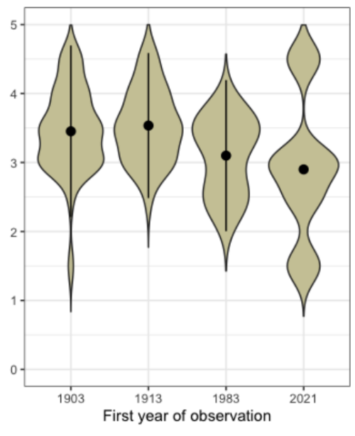
To our surprise, our research uncovered some unexpected findings. Using historical botanical records from 1903, 1913, and 1983, along with our own resurvey in 2021, we were able to partially reconstruct the long-term dynamics of these species. We initially hypothesized that the low levels of non-native ruderal species observed today indicated that their introduction was relatively recent, likely after the construction of the main highway (the ‘E10’ in the 1980s, compounded by increased tourism and climate change in recent decades.
Our historical sources tell an entirely different story, however. Many ruderal species were already present and common during the creation of the Rallarvägen. Remarkably, there were even more non-native species back then than there are now, and we have observed a consistent decline since then. Even more surprisingly, this decline has led to the current ruderal community having fewer warm-adapted species than during the era of railroad construction. This implies that warm-adapted species are disappearing rather than emerging. This pattern holds true for both native and non-native ruderals.
A remarkable decline in warm-adapted non-native species over time, as reflected by the range of ‘temperature indicator values’ by all species in each of the survey years.
The conclusion is clear: a major historical disturbance, such as the construction of the railroad back in 1903, can send shockwaves through an ecosystem that are still felt a century later. In this case, the impact of that disturbance has been even greater than that of contemporary climate change, as evidenced by the decline in both species richness and the temperature affinity of the community over time.
Our historical data is incomplete, so there remains some uncertainty about the exact sequence of events. Nonetheless, we could piece together a remarkable history that begins with gardens, stables, and foreign soil filled with ruderal seeds, followed by a steady decrease in disturbance levels and a corresponding decline in non-native ruderal species richness. The construction of the highway in the 1980s and its use since then has not yet resulted in an increase in ruderals along the Rallarvägen, likely because the Rallarvägen was not used as a construction road for the building of the highway. Nor has the recent warming climate led to a resurgence of these species.
Nowadays, ruderal species are as expected most strongly related to hotspots of introductions, such as the small train stations scattered along the tracks. Interestingly, here again disturbance trumps climate: the relationship of ruderal species was much stronger with disturbance than with climate.
A final interesting observation to point at here is that only very few ruderals, and especially non-native ruderals, have found their way from the Rallarvägen in the valley to higher elevations. Despite the presence of some well-visited hiking trails crossing the Rallarvägen, the uphill expansion of non-natives is limited. That is remarkable, given that they have had more than a hundred years to do so. The conclusion should thus be that most of these species are currently truly at their climatic limits here in the high north. Only a change in climate could thus make them move higher up…
Let that unfortunately exactly be what is happening…
It has become the go-to technique for many ecologists who need a cheap and simple method to measure decomposition rates in the soil: burying tea bags. However, it is still rather mindboggling that the team behind the international Tea Bag Index collected data from 36.000 (!) of these cups of soil tea from across the globe. The key conclusions from this monitoring project with perhaps one of the more unusual sources of data in ecology (although clearly rivaled by ‘operation underpants’, where underwear is used for the same purpose) now got published in Ecology Letters. As contributor of my own set of these brews to the mix, I happily took part in this endeavor.
A pile of tea bags, ready to be buried for science
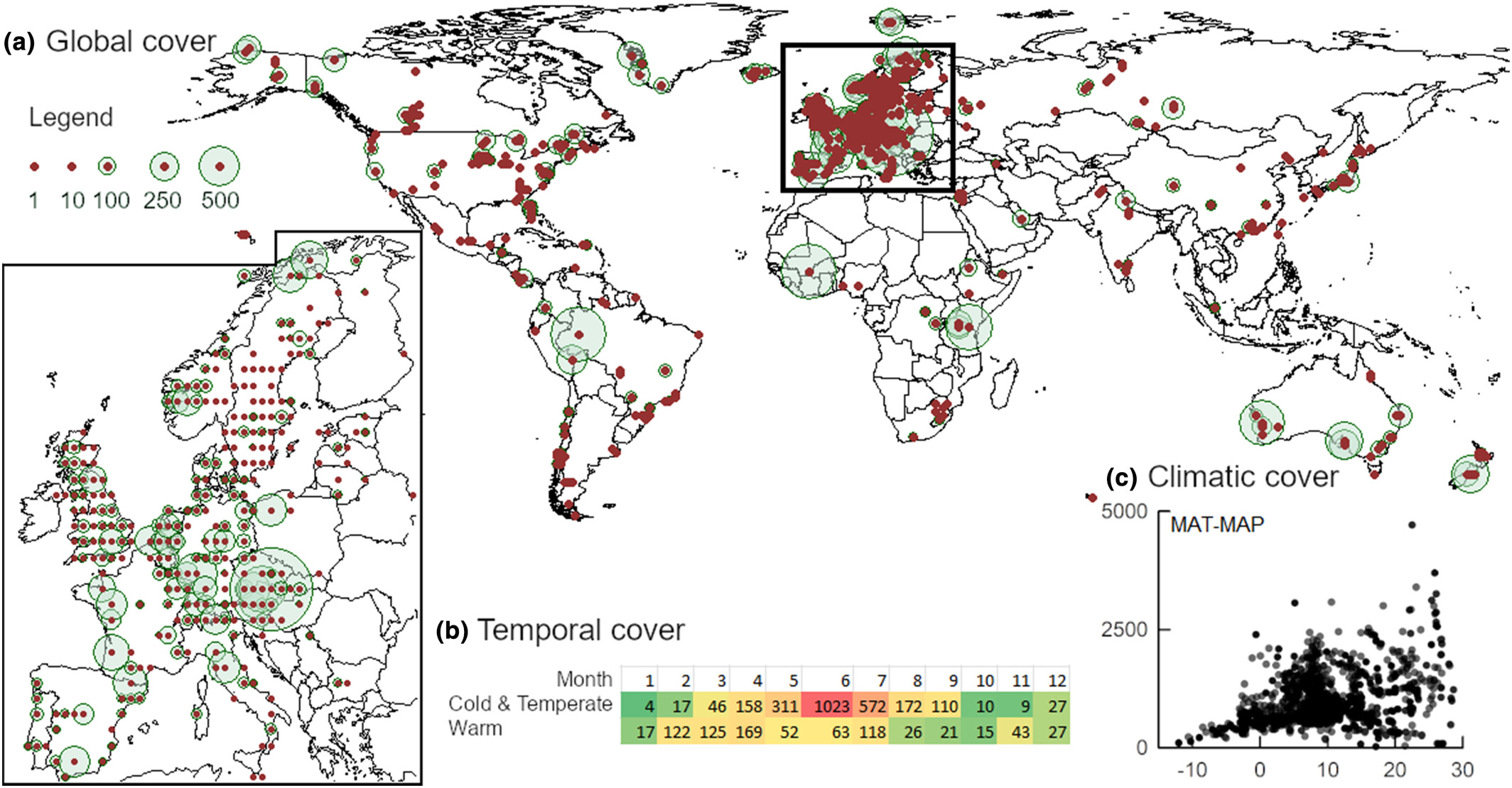
Burying tea bags is appealing for two reasons: you know the litter type, and you know the exact quantity of it. Standardizing both across all of the worlds’ soils can provide a unique insight in differences in the rate of decomposition across these soils. Indeed, for a fair comparison of litter decomposition, one needs to standardize the type and quantity of buried plant material. The choice of Lipton tea bags, consistent in plant species and weight worldwide, resolved this methodological challenge.
The global spread of the mindboggling 36.000 tea bags
The study participants buried both the very leafy green tea and the more recalcitrant rooibos tea. After a predetermined time, the partially decomposed tea bags were excavated and weighed to ascertain weight loss. Subsequent analyses aimed to disentangle the influence of climate variations and anthropogenic land use on both decomposition rates and the extent of material breakdown (and thus the resulting stabilization of the remaining material).
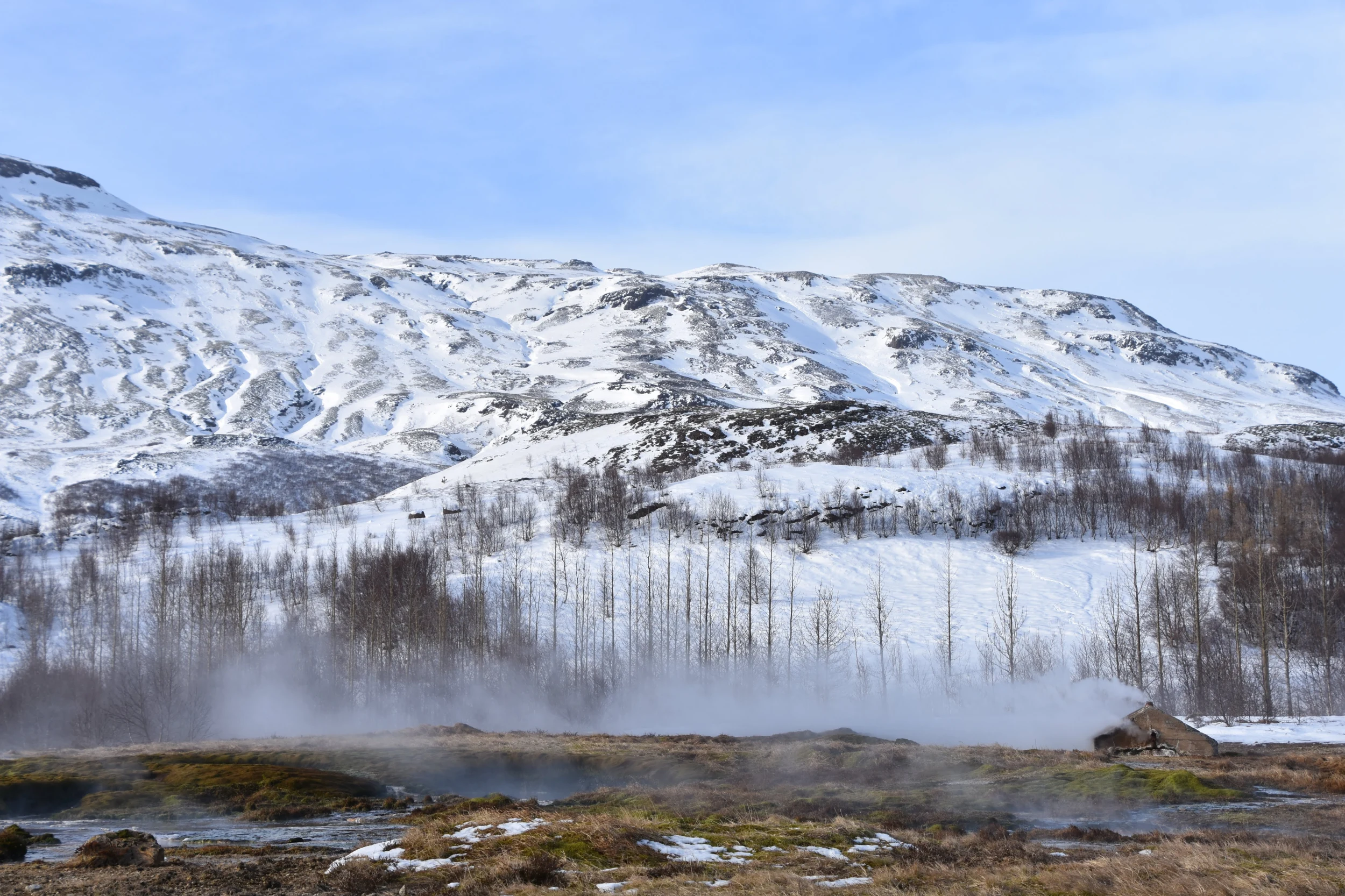
Tea bag decomposition is strongly influenced by local climate conditions (which are rather unusual in the depicted Icelandic landscape).
One would hypothesize that the initial rate of decomposition and the amount of mass loss correlate pretty well at a global scale. Using our thousands of tea bags, we found this to be true, indeed, yet with some intriguing nuances, particularly in cold regions, where decomposition dynamics defied conventional expectations.
Indeed, especially in cold regions, we often observed initially relatively quick breakdown of a portion of organic material, yet high remaining mass loss. This mismatch between loss rate and stabilisation is important, and could for example result from different drivers of two main competing pathways responsible for said mass loss: simple leaching of soluble components into the soil, versus breakdown by soil microbes. While the latter is rather sluggish in cold environments, the former can still result in rapid mass loss. While our correlational study cannot be conclusive regarding the exact driver at play – and we discuss some alternative hypotheses in the text – these findings do underscore the intricate region-specific complexities of these biogeochemical processes.
Global patterns in mass loss rates (kTBI) and stabilisation (STBI) as modelled using the 36.000 tea bags. Bottom panels indicate areas with lower accuracy (higher CoV).
In conclusion, our study sheds light on the intricate relationship between climatic factors and litter decomposition rates, emphasizing their vital role in ecosystem carbon cycling, particularly in the face of climate change. By uncovering context-dependent effects, we highlight the need for nuanced approaches in global carbon modeling. Our findings underscore the significance of empirical data in refining our understanding of these complex dynamics and in improving the accuracy of carbon models.
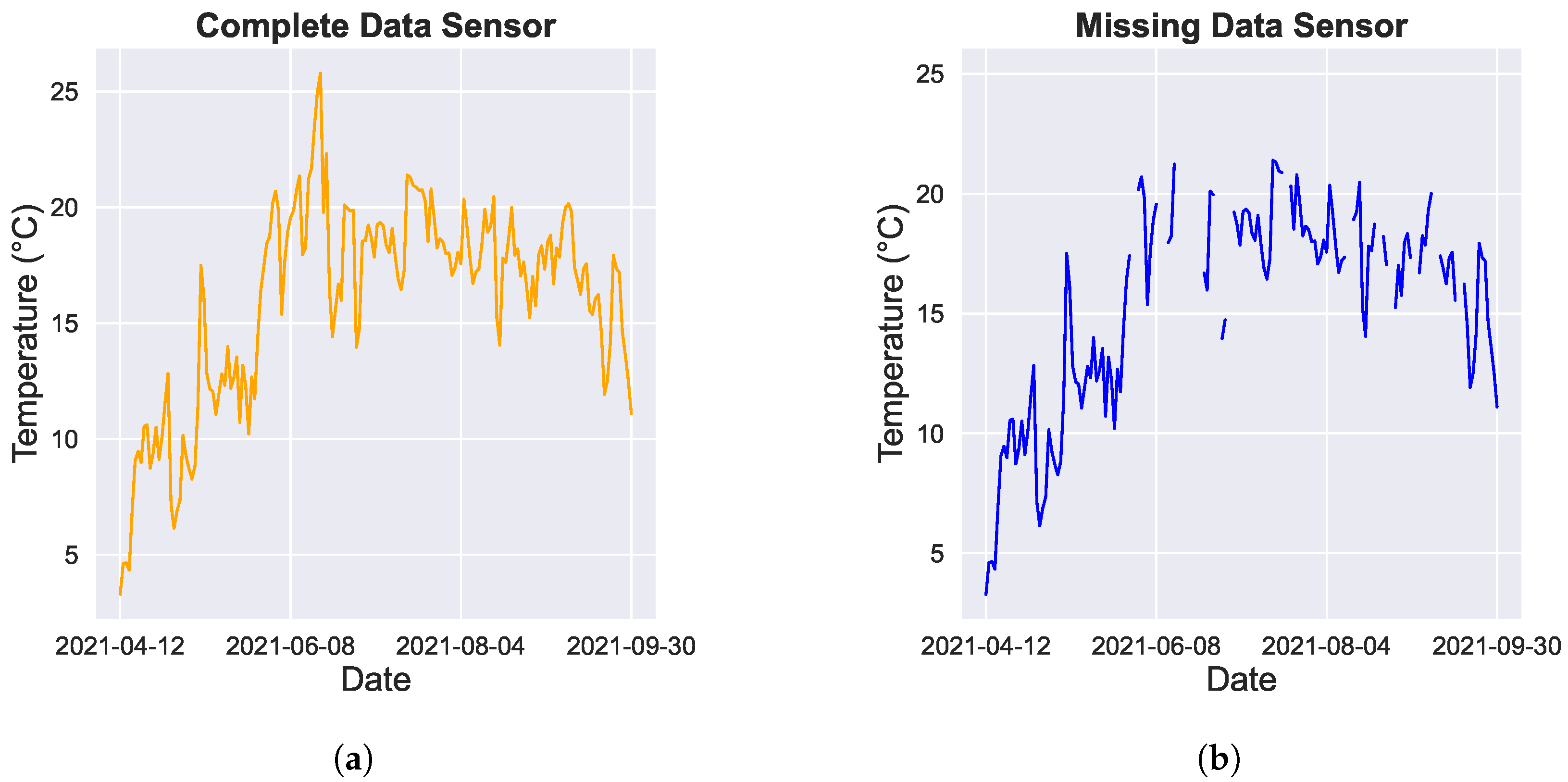
Anyone working with microclimate data is familiar with time series data – repeated measurements over time at the same location.
And anyone working with time series has bumped into an important potential issue with them: gaps. More often than not, time series are incomplete. There could be erroneous measurements, sensor malfunctioning, sensor replacement, data transfer issues, memory issues and so on.
Over time, a whole toolbox of techniques has emerged to fill those gaps and make those time-series whole again. In a recent paper, we tested a series of these gap-filling methodologies for their accuracy. That question is important especially for microclimate networks, as here not only the temporal but also the spatial relationship between time series is playing a role, and filling gaps is thus not a trivial exercise.
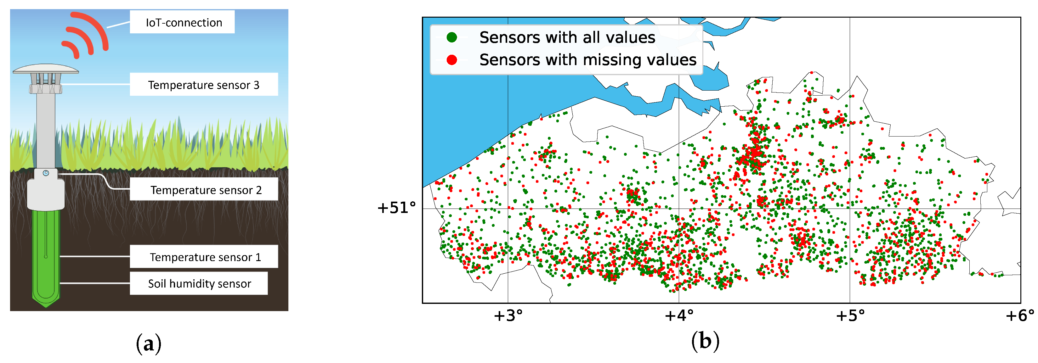
In this paper, we applied and evaluated 12 such gap-filling methods to complete the missing values in a dataset originating from large-scale environmental monitoring. For this, we used the unique dataset of 4400 IoT-connected microclimate sensors that were deployed across Flanders as part of ‘CurieuzeNeuzen in de Tuin’, our large-scale citizen science project on heat and drought.
(a) The TMS-NB microclimate sensor was used in a large-scale citizen science project on microclimate monitoring. The sensor measures temperature at three heights, as well as soil moisture. Data transmission occurred via NB-IoT. (b) The WSN covered 4400 gardens across Flanders. Sensor locations are colored based on whether time series were complete (green) or had missing records (red).
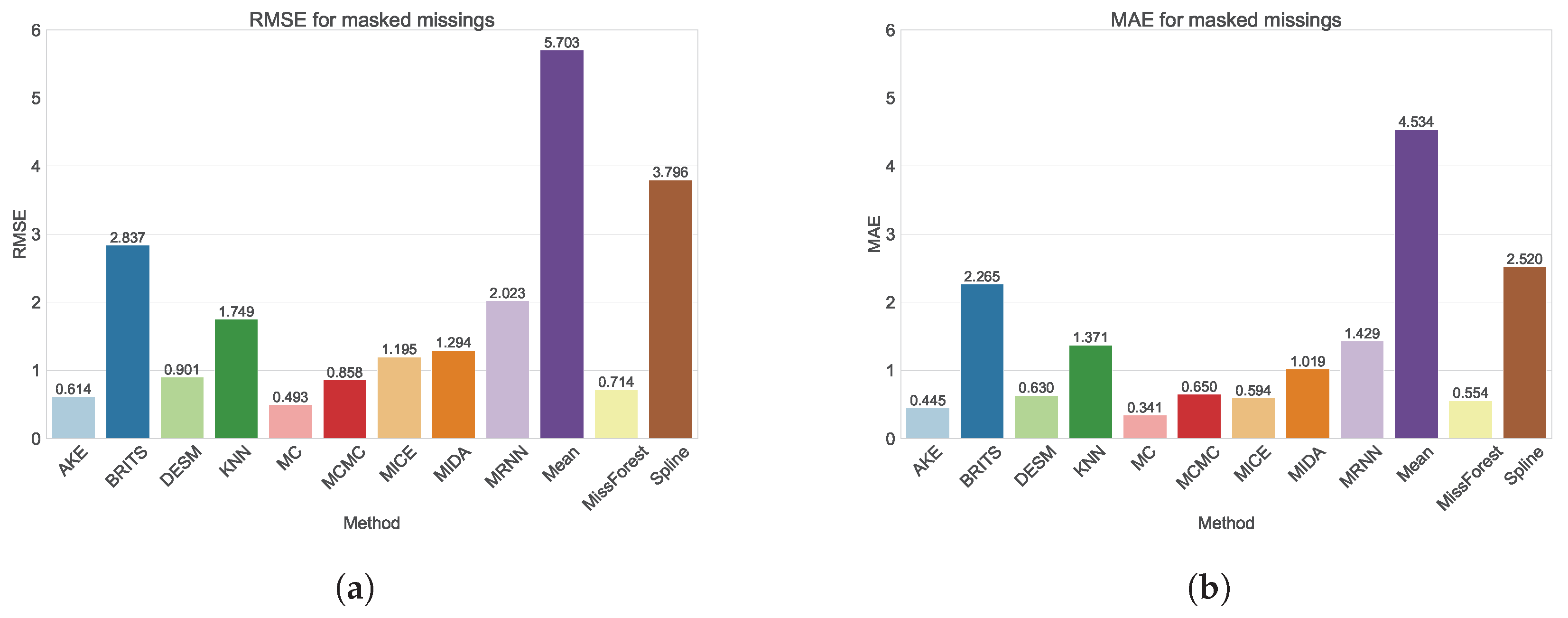
Methods evaluated included Spline Interpolation, MissForest, MICE, MCMC, M-RNN, BRITS, and others, and the performance of these imputation methods was evaluated for different proportions of missing data (ranging from 10% to 50%), as well as a realistic missing value scenario.
Accuraccy estimates (Root Mean Square Error and Mean Absolute Error) for the twelve tested imputation methods
Interestingly, techniques leveraging the spatial features of the data (such as MC, MCMC and MissForest in the graph above) tended to outperform the time-based methods. Importantly, as well, real scenarios of missing values – with gaps often occurring in larger blocks – often resulted in a lower performance of the models than artificial scenarios with randomly missing points, especially for more traditional techniques such as MICE.
Of course, this result is not the final conclusion on the debate which gap-filling technique to use. The outcome strongly depends on the specifics of the datasets at hand, in our case a dataset of microclimate data of fairly short duration (only little seasonality), with relatively sparse temporal resolution (every 15 minutes) and unusually high spatial density (4400 sensors across Flanders). These features work in favour of techniques that take the spatial features of the data into account, and reduce the applicability of e.g., deep-learning techniques that might prove more robust for more complex time series with longer temporal window and higher temporal resolution.
So, let’s hope this exercise in gap-filling can help other microclimate enthusiasts in their search for good solutions!
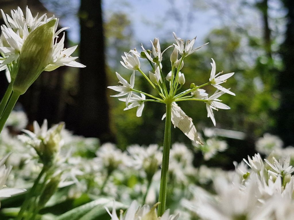
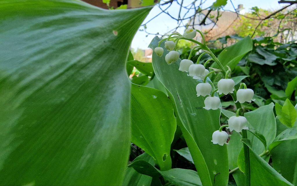
One could wonder if the microclimate-based models of Haesen et al. would have predicted such a wealth of wildflowers in the garden of our new home!
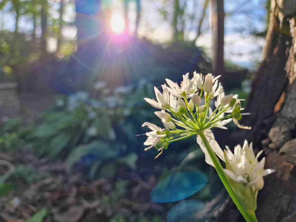
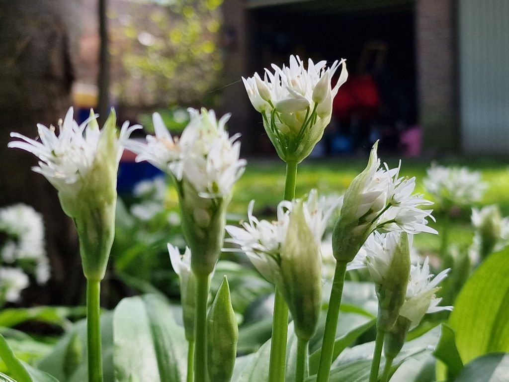
Wild garlic
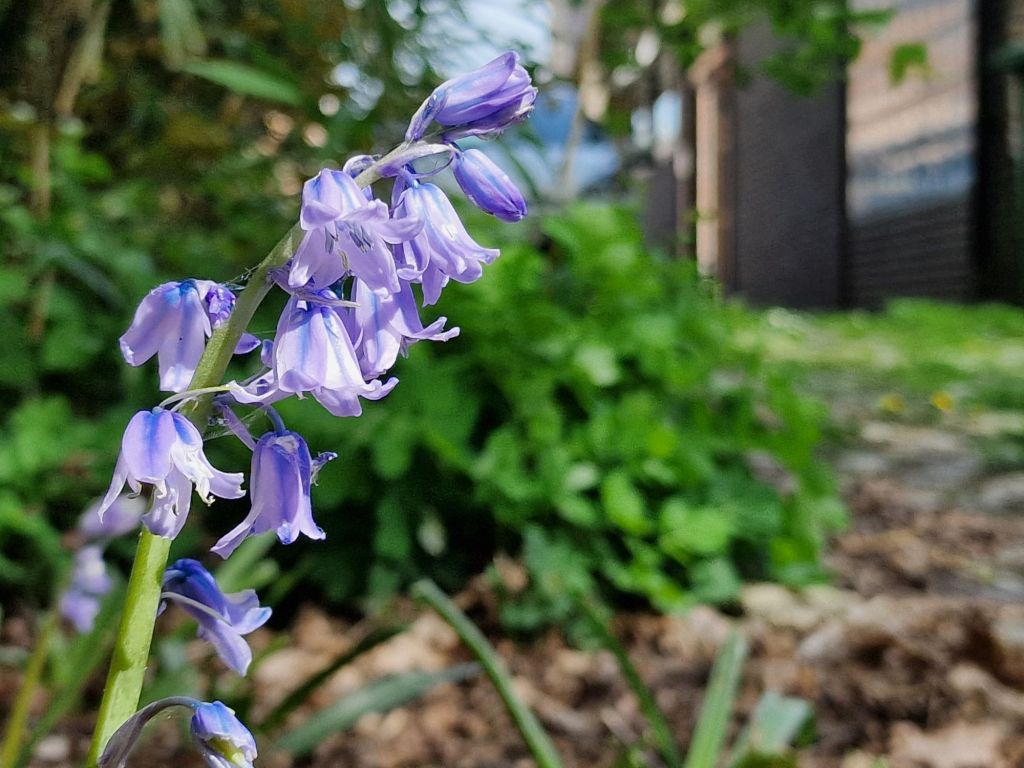
This is our first spring in our new garden, and we could thus have hardly foreseen that so many beautiful decorations would spring up in our little patch of forest!
Lily of the valley
Of course, that is if our distribution models would not have said so. In this recent paper in Ecology Letters, we used our high resolution (5 x 5 m) maps of forest microclimate to improve distribution models of forest understory plants.
5 x5 m might just be enough to give our garden its own little pixel on the maps, so it could be worthy to investigate…
Of course, I should not tell you that all that greenery was one of the reasons why we bought the place, so I am beyond excited that the garden is rewarding our decision so handsomely!
Angelica archangelica along mountain road in the northern Scandes, Norway
Skjomen valley, northern Norway
Narvik, Norway
Trifolium repens
Lake Torneträsk, Abisko, Sweden
Narvik, Norway
Narvik, Norway
Abisko, Sweden
Oenanthe oenanthe
Skjomen valley, northern Norway
Luscinia svecica
Norway, Narvik
Narvik, Norway
Diapensia lapponica in one of our plots
Skjomen valley, northern Norway
Norway
Hallerbos 2017
Young bluebell (Hyacinthoides non-scripta) surrounded by flowers of yellow archangel (Lamium galeobdolon)
The common bluebell (Hyacinthoides non-scripta), the signature flower of the Hallerbos
Single bluebell flower surviving on a wetter spot, as indicated by the field of wild garlic (Allium ursinum)
A really wet patch of forest, with giant horsetail (Equisetum telmateia) in a field of wild garlic (Allium ursinum)
Wild garlic (Allium ursinum) in the Hallerbos flowers a bit later than the bluebells, yet this one was already in full bloom
A bumblebee visiting yellow archangel (Lamium galeobdolon)
A bumblebee visiting yellow archangel (Lamium galeobdolon)
Wild garlic (Allium ursinum)
Wild garlic (Allium ursinum)
Weirdly beautiful, the inflorescence of pendulous sedge (Carex pendula), typical for the wettest spots in the forest
Weirdly beautiful, the inflorescence of pendulous sedge (Carex pendula), typical for the wettest spots in the forest
A little stream in the Hallerbos, surrounded by endless fields of wild garlic (Allium ursinum)
The herb-paris (Paris quadrifolia), less common in the forest
Wild garlic (Allium ursinum)
Bluebells (Hyacinthoides non-scripta)
Weirdly beautiful, the inflorescence of pendulous sedge (Carex pendula), typical for the wettest spots in the forest
Another one from the wet plots: large bitter-cress (Cardamine amara)
Another one from the wet plots: large bitter-cress (Cardamine amara)
Young beech leaves, as soon as they are fully grown, spring in the understory is over
A beech forest without understory, most likely too dry and too acid for any survivors
A young beech seedling (Fagus sylvatica), looking nothing like a beech, yet everything like a tiny dancer
Young beech seedling (Fagus sylvatica)
Bluebells (Hyacinthoides non-scripta)
Bluebells (Hyacinthoides non-scripta)
Bluebells (Hyacinthoides non-scripta)
Mountain melick (Melica nutans), a grass in the most amazing green
Bluebells (Hyacinthoides non-scripta) in a rare patch of mountain melick (Melica nutans), a grass in the most amazing green
Bluebells (Hyacinthoides non-scripta)
Bluebells (Hyacinthoides non-scripta)
Montpellier 2017
The entrance to the cathedral of Montpellier
The cathedral of Montpellier
The entrance to the cathedral of Montpellier
The cathedral of Montpellier
Narcissus poetics
The cathedral of Montpellier
The botanical garden of Montpellier
The botanical garden of Montpellier
The botanical garden of Montpellier
Brackish Camargue vegetation
Brackish Camargue vegetation
Brackish Camargue vegetation
A typical lagune
Brackish Camargue vegetation
Camargue horses
Camargue horses
Camargue horses
Brackish Camargue vegetation
Brackish Camargue vegetation
Brackish Camargue vegetation
Camargue horses
Brackish Camargue vegetation
Little egret in the evening sun
Flamingo’s in the evening sun
A typical lagune
Dandelion fuzz
Grass lily
Grass lily
Dandelion fuzz
Veronica in a sea of poplar fluff
Euphorbia in a sea of poplar fluff
Poplar
Gare du Midi, Brussels
Gare du Midi, Brussels
Gare du Midi, Brussels
Gare du Midi, Brussels
Sweden autumn 2016
Autumn in Abisko
Yellow leaves of mountain birch, with lake Torneträsk in the background.
Lapporten, the gate to Lapland, in Abisko
Rain blowing over the Abisko National Park
The colours of the north: red fireweed and yellow mountain birches, with lake Torneträsk on the background
Yellow leaves of mountain birch, with lake Torneträsk in the background.
Rain on the background, the ski lift in Abisko on the foreground
The steep slope of mount Nuolja on a dramatic looking morning
The beautiful colors of lake Torneträsk in Abisko
A little stream on top of the mountain, with a view on Lapporten, the gate to Lapland
Well, that is a beautiful table with a nice view on lake Torneträsk in Abisko
Our little experiment on top of the mountain in Abisko, with a view on Lapporten
Autumn in Abisko is extremely colorfull
The ski lift with a view on Abisko National Park and Lapporten
Hiking dowhill towards lake Torneträsk
This green is greener than the greenest green: moss on top of mount Nuolja
Well, that is a beautiful table with a nice view on lake Torneträsk in Abisko
The ski lift with a view on Abisko National Park and Lapporten
The ski lift with a view on Abisko National Park and Lapporten
The most beautiful hiking trail of the world: Nuolja in Abisko
Angelica archangelica, often the biggest plant of the Arctic
The most beautiful hiking trail of the world: Nuolja in Abisko
Cirsium helenioides, the melancholy thistle
Hiking down mount Nuolja
The steep slope of mount Nuolja on a dramatic looking morning
The colours of the north: red fireweed and yellow mountain birches, with lake Torneträsk on the background
The prettiest yellow and blue: autumn in Abisko
Fireweed, Epilobium angustifolium
Campanula or bellflower, I think ‘uniflora’
Vaccinium myrtillus
Cornus suecica, the prettiest red of the world
Hieracium alpinum, alpine hawkweed
Carex atrata, one of my favourite sedges
Alpine clubmoss, Diphasiastrum alpinum
Agrostis capillaris, bentgrass
Common yarrow (Achillea millefolium)
Anthoxanthum odoratum, sweet vernal grass, fully grown and mature
Snow scooter trail
Our plot in the mids of a field of horsetails (Equisetum pratense)
Equisetum pratense
Cliff overlooking the valley with the road to Norway
Seedling of Taraxacum officinale, the dandelion, after two years of growing in bad conditions
Poa alpina, the alpine meadow-grass, with its viviparous seeds
Massive flowerhead of Angelica archangelica
Angelica archangelica
Blueberry (Vaccinium myrtillus) in autumn
A lowland marsh in Abisko in autumn
Installing the plots of our trail observations on top of mount Nuolja
Installing the plots of our trail observations on top of mount Nuolja
Tanacetum vulgare (Tansy), non-native for the high north
Autumn forest down in the valley
The valley of Nuolja to Björkliden
Summer on the Nuolja-side
A full rainbow behind mount Nuolja in Abisko
It’s raining in the west, clouds trapped behind the mountains
A strong wind blowing rain from behind the mountains to our side
A strong wind blowing rain from behind the mountains to our side
Betula nana, the dwarf birch, mini autumn forest
Betula nana, the dwarf birch, mini autumn forest
The valley of Björkliden in autumn
The valley of Björkliden in autumn
The valley of Björkliden in autumn
The valley of Björkliden in autumn
Sweden spring 2016
Oxyria digyna
Although the alpine zone has been harder for invasives to access than most places, human structures like trails are often an easy gateway for the invaders to get up there. Picture from Abisko, Swedish Lapland.
Eriophorum vaginatum
Silene suecica
Ranunculus glacialis
Trifolium pratense
Salix reticulata
Silene acaulis
Rubus arcticus
A rainy hike
The valley of the lakes
Cornus suecica
Western European species like the red clover (Trifolium pratense) here are often listed as non-native species in mountain regions.
Bartsia alpina
Trifolium repens
Melting snowpatch on a lake
Overlooking the valley of Laktajakka
Dryas octopetala
Ranunculus glacialis
Amiens
Colourful mirror
Cathedral with a glimpse of spring
Almost cold enough for ice-skating
Sunny but cold, the Quai Bélu
Amiens is filled with cute little houses
View from my office window
The southern side
Frozen mirror
Frozen to the bone
Cathedral at night
The museum behind the beautiful gates
House on the square before the cathedral
Cathedral at night
Sun rising above the water
Gargoyle planning to eat the cathedral
Enjoying silence and the morning sun
Le Club d’Aviron in winter weather
Cold!
View from my office window
Just outside of Amiens
Winter sun on the Place du Don
Cathedral at night
Nice architectural curve
Cathedral seen from the frozen Parc Saint-Pierre
Sunny but cold, the Quai Bélu
Maria without a shirt
Cathedral at night
Sweden autumn 2015
Lichen
Sweden summer 2015
View on the 1000 meter plots
Doing research on a cold Arctic morning
Plots flooded by the snowmelt
Flooded by the snowmelt
Meltwater river, racing down the mountain
After a hike, even the most basic house looks cosy. Little hut in the mountains, open for everybody
Snowbridge, maybe don’t cross…
Snowbridge
View from a cliff
Silene acaulis or cushion pink, cutest plant of the Arctic
Two seasons in one image
Steep slope
Hiking down
Narvik Kirche, church of the subarctic
Narvik Kirche
Reindeer on top of the mountain
Narvik Kirche
Summer at the church
Summer flowers
Massive waterfall
Young willow catkins
View from Narvik’s hospital, with lilac flowers
Building a bridge over the fjord will gain al drivers at least an hour
Norwegian fjord
Posing with the water, getting soaked
Minimalistic mountains
Insect investigating our reindeer antler
Catching mosquitoes with our license plate, harvest of the year!
Posing with the plot
Fieldwork on the most beautiful spot of the world
Fieldwork on the most beautiful spot of the world
Summer bridge – still next to the sadly impassable river
Rhinanthus flower in the mountains
Plateau in the valley, beautiful brown
Experimental view from my favourite plot
Salix catkins
Extremely old Betula tree
Waterfall from a cliff
Buttercup is the earliest in spring, here
Rocks!
Alpine views
Views!
Fieldwork
Jumping over rivers
Plot
Golden plover
Angry lemming
Green, the whole north is green!
Snow, so much snow left!
Minimalistic mountain moments
Fieldwork
The research center
Red clover – focal invader
Look at this tiny cute snail!
Massive floods of melting water
Bartsia alpina
Hooray, a toilet!
Dryas octopetala
Lowest elevation plots
Butterball!
That’s a lot of water
Midnight sun is the best
At the lakeside
Beautiful Bistorta vivipara
Don’t fall in the water
Midnight sun
Wild river
Art – made by ages of wild rivers
Baby firework for America’s independence day
Midnight sun at the lake
The Abisko canyon was wilder than ever
That’s a crazy amount of water!
The Abisko canyon was wilder than ever
The Abisko canyon was wilder than ever
Black and white
Stone-man overlooking Abisko
Nothing as soft as a willow catkin
Label and soil temperature sensor attached
I’d drive to the top every day
Reflections
Rocks and clouds
Brave little birch
Brewing our camping poison
Basic camping stuff
Camping in Norway
Home-made temperature houses
Roadside research at its best
Norway is crazy
Horsetail is so funny
Little creek in magical forest
Birches, birches everywhere
Beautiful rock, a gift from the river
Another roadside fellow
Lichen
Ready to rock the summer
Collecting mosses
That’s a crazy old lichen
Tiny tiny piny trees, but old, so old!
Ready to jump into the fjord?
Ready to jump into the fjord?
That’s a spiky stone!
Views on Norwegian fjords
Silene in the mountains
Cute little orchid
Skua
Attacking skua, mind your heads!
Watch out for the attack of the fierce skua!
Black snail
New plot!
Still a lot of snow to melt, but this spot was free for a new plot
Reindeer are better than people
Two seasons in one picture
Let’s see what is happening to the balance in mountains! Is this a starting avalanche, or will it last a bit longer?
Cute little hut
Climbing mountains by car
Softest moss in history
Drosera in the marsh
Hiking in no-man’s land
The clouds are coming
Abisko valley
‘Butterball’
Fieldwork in the tundra
Abisko valley
Little plot
Clouds and sun and mountains
Making soup on a campfire with a view
Little creek on high elevations
Skua on the look-out
Melting snow in a river
Rhodiola rosea and the Törnetrask lake
Beginning of spring
Flooded plots, melting snow, impassible wetness
Ferns and horsetails
Chile 2015
Lunch made by our local colleague, with funny bread (tasty as well!)
Trips to the field sites were sometimes a real adventure, especially right after snowmelt


")


")
")


")


")


")


")


")


