
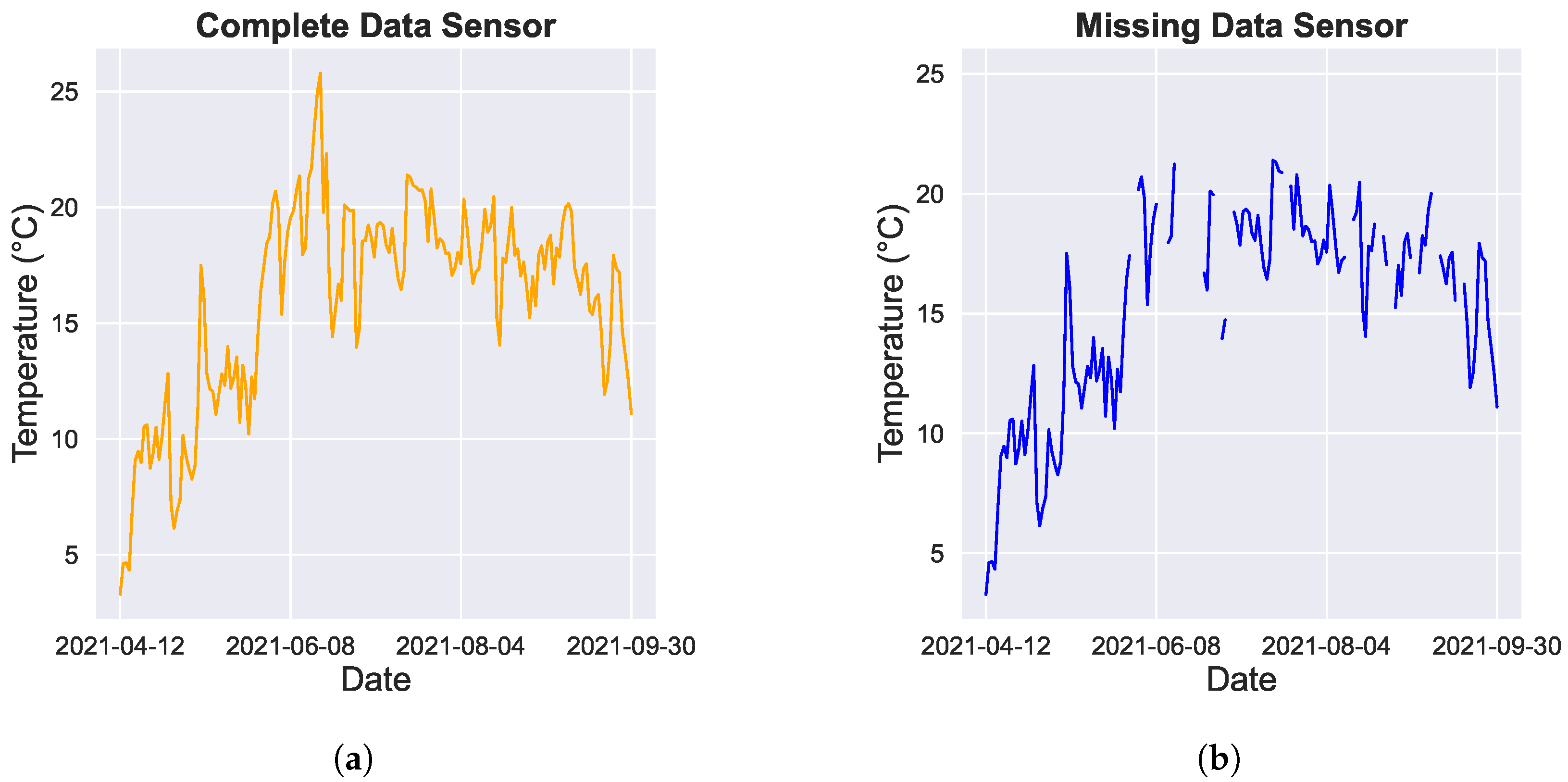
Anyone working with microclimate data is familiar with time series data – repeated measurements over time at the same location.
And anyone working with time series has bumped into an important potential issue with them: gaps. More often than not, time series are incomplete. There could be erroneous measurements, sensor malfunctioning, sensor replacement, data transfer issues, memory issues and so on.
Over time, a whole toolbox of techniques has emerged to fill those gaps and make those time-series whole again. In a recent paper, we tested a series of these gap-filling methodologies for their accuracy. That question is important especially for microclimate networks, as here not only the temporal but also the spatial relationship between time series is playing a role, and filling gaps is thus not a trivial exercise.
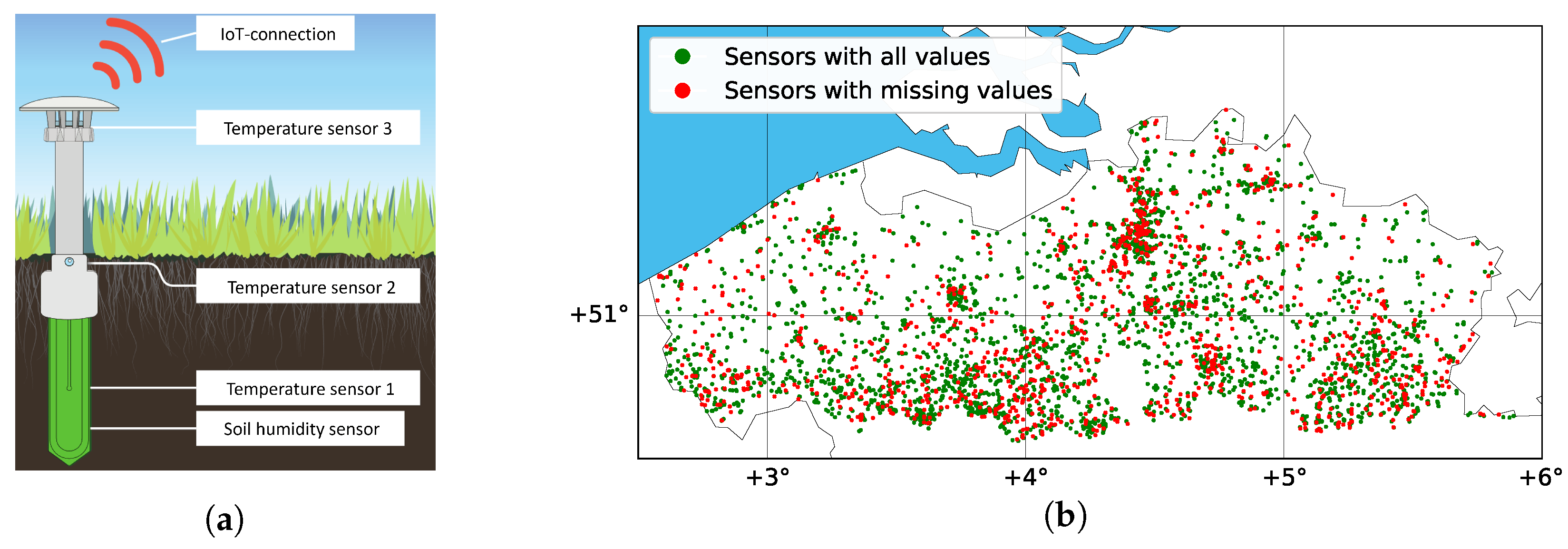
In this paper, we applied and evaluated 12 such gap-filling methods to complete the missing values in a dataset originating from large-scale environmental monitoring. For this, we used the unique dataset of 4400 IoT-connected microclimate sensors that were deployed across Flanders as part of ‘CurieuzeNeuzen in de Tuin’, our large-scale citizen science project on heat and drought.
Methods evaluated included Spline Interpolation, MissForest, MICE, MCMC, M-RNN, BRITS, and others, and the performance of these imputation methods was evaluated for different proportions of missing data (ranging from 10% to 50%), as well as a realistic missing value scenario.
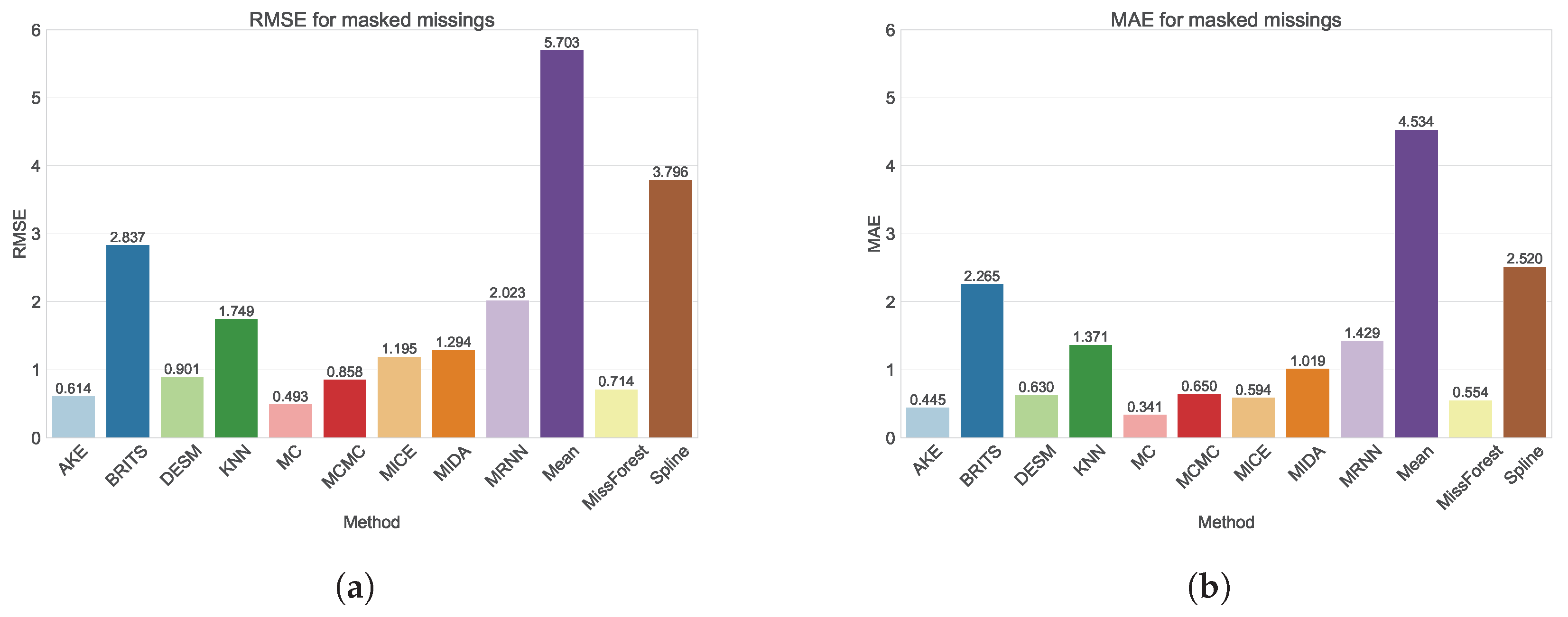
Interestingly, techniques leveraging the spatial features of the data (such as MC, MCMC and MissForest in the graph above) tended to outperform the time-based methods. Importantly, as well, real scenarios of missing values – with gaps often occurring in larger blocks – often resulted in a lower performance of the models than artificial scenarios with randomly missing points, especially for more traditional techniques such as MICE.
Of course, this result is not the final conclusion on the debate which gap-filling technique to use. The outcome strongly depends on the specifics of the datasets at hand, in our case a dataset of microclimate data of fairly short duration (only little seasonality), with relatively sparse temporal resolution (every 15 minutes) and unusually high spatial density (4400 sensors across Flanders). These features work in favour of techniques that take the spatial features of the data into account, and reduce the applicability of e.g., deep-learning techniques that might prove more robust for more complex time series with longer temporal window and higher temporal resolution.
So, let’s hope this exercise in gap-filling can help other microclimate enthusiasts in their search for good solutions!


")


")
")


")


")


")
")


")


